Jonathan Capone — Mission Portal & AI

Spatial Computing

The Glass Bridge Interface.

The Mission Portal is a ~52,500 LOC Vanilla JS workbench built for high-performance 3D visualization. It renders 79 distinct layer profiles and 10 animated 4D Copernicus fields over a shared design system. The base layer is a 3D WebGL globe (powered by Deck.gl/CesiumJS) that occupies 100% of the viewport. There are no permanent sidebars.

Instead of cluttered UI panels, OMEGA utilizes Contextual Progressive Disclosure. Tools and data panels live in floating "context drawers" that slide into the viewport only when a user selects a specific entity (like a buoy or a drawn polygon). Clicking the open ocean dismisses the drawer entirely.

Global State

4D Temporal & Z-Axis Engine.

The ocean is a 4D volume. The entire application operates on a single synchronized state across time, X, Y, and Z axes.

Time

Master Time Clock

Scrubbing the timeline backward pauses live WebSocket streams and simultaneously queries historical databases for local telemetry, ocean physics (Copernicus), and redraws the exact active mesh topology for that specific second.

Depth

Z-Axis Slicer

A persistent depth slider allows operators to slice from 0m down to -2000m. Doing so dynamically updates colormaps and thermoclines on the 3D globe—treating the ocean as a true volumetric data cube.

Visual Ontology

Absolute Data Purity.

The core prime directive of the DTO v3.0 interface is Absolute Data Purity. The system must NEVER use modeled API data to fill gaps in the physical hardware's dataset. Missing telemetry is rendered explicitly as a visual gap.

To enforce this, the UI employs a strict visual ontology: Ground Truth from the physical mesh is rendered as sharp, high-contrast, opaque 3D geometry (extruded columns and hard-edged pins). Modeled Data from APIs (like Copernicus winds and currents) are rendered using GPU particle shaders, dynamic colormaps, and semi-transparent volumetric layers.

Routing

Operational Workspaces.

The portal is divided into dedicated workspaces tailored for specific mission phases.

/observe

Live Observatory

Features 3D particle physics powered by GPU shaders to animate wind and currents, a living mesh visualizer drawing topological links (LoRa/JANUS), and a contextual QARTOD lens for anomaly verification.

/plan

Predictive Simulation

A Particle Dispersion Engine simulating spills and passive drifters using 7-day current forecasts, alongside a kinematic hazard engine cross-referencing hardware capabilities against AIS traffic and GEBCO bathymetry.

/analyze

Data Library

A standalone data lab allowing operators to filter, rank, and correlate ground truth against historical API models, and upload offline CSV/GeoJSON logs without polluting the live operational database.

/admin

Engineering Deck

Behind strict administrative authentication. Controls hardware configuration, gateway runtime toggles, HaLow AP/STA pairing, and API credential loading.

/public

Public Federation

A read-only mode with command and routing tools disabled. Designed as a safe URL state for classrooms and researchers to view live telemetry and interact with 3D environmental visualizations.

State Decoupling

Digital Twins & UI State.

Because edge nodes operate on aggressive battery-saving duty cycles, they are often offline and entirely uncontactable for hours at a time. Therefore, the frontend cannot assume that clicking a "Format NVRAM" button instantly formats the storage.

To solve this synchronization gap, OMEGA models all physical assets on the map as Digital Twins. The UI manages strictly decoupled state variables for every user action: pending (the operator clicked the button in the UI), synced (the shore gateway queued the command into the DTN mesh), and reported (the hardware edge node physically acknowledged the change and beamed the result back).

web/src/types/MissionState.ts

export type SyncStatus = 'pending' | 'synced' | 'reported' | 'failed';

export interface DigitalTwinCommand {
  command_id: string;
  target_node: string;
  intent: string;
  payload: any;
  
  // Tripartite State Tracker
  // pending: UI clicked, waiting on network
  // synced: Shore gateway confirmed receipt
  // reported: Physical edge node confirmed execution over LoRa
  status: SyncStatus;
  
  timestamps: {
    requested_at: string;
    synced_at?: string;
    reported_at?: string;
  };
}

Mathematical Signal Processing

QARTOD Quality Control Math.

The gateway/analytics.py engine is the mathematical workhorse of the shore system. It constantly crunches millions of historical SQLite telemetry points using strict QARTOD (Quality Assurance / Quality Control of Real-Time Oceanographic Data) standards.

Spike Detection via First Derivative: When a hydrophone passes a thermocline, it might record a massive, legitimate spike in temperature (an ocean front). Standard deviation checks would flag this as an error. OMEGA uses the mathematical first derivative test: |V2 - V1| - |V3 - V1| / 2 > Spike_Threshold. This equation proves whether a sudden spike mathematically returned to the baseline (a sensor glitch) or established a new baseline (a legitimate oceanographic event).

Gross Range Processing: For localized anomalies, the numpy arrays execute vectorized operations using the Median Absolute Deviation (MAD): MAD = median(|Xi - median(X)|). Because standard averages are destroyed by massive outliers, the MAD provides an unbreakable center. If a value exceeds MAD * 1.4826 * 3, it is flagged as suspect. At 6 sigmas, it is stripped from the DOM.

gateway/qc.py

def _threshold_bundle(values: list[float]) -> dict[str, float] | None:
    # Calculate QARTOD compliant statistical bounds
    center = np.median(values)
    mad = np.median(np.abs(values - center))
    robust_sigma = mad * 1.4826
    
    return {
        "gross_range_suspect_min": center - robust_sigma * 3,
        "gross_range_suspect_max": center + robust_sigma * 3,
        "gross_range_fail_min": center - robust_sigma * 6,
        "gross_range_fail_max": center + robust_sigma * 6,
    }

gateway/analytics_merge.py

import pandas as pd
import sqlite3

def build_multivariate_dataset(db_path: str):
    """
    Oceanographic sensors sample at different frequencies. 
    Temperatures arrive every 15m; Salinity arrives every 1h.
    We must use Pandas merge_asof() to align time-series backward 
    in time to the nearest exact sample, avoiding future-data leakage.
    """
    conn = sqlite3.connect(db_path)
    
    # Load raw telemetry into DataFrames
    df_temp = pd.read_sql("SELECT timestamp, temperature FROM telemetry", conn)
    df_salt = pd.read_sql("SELECT timestamp, salinity FROM telemetry", conn)
    
    # Sort by time required for asof merge
    df_temp.sort_values("timestamp", inplace=True)
    df_salt.sort_values("timestamp", inplace=True)
    
    # Merge Salinity to Temperature, looking backward up to 2 hours
    df_merged = pd.merge_asof(
        df_temp, 
        df_salt, 
        on="timestamp", 
        direction="backward",
        tolerance=pd.Timedelta("2h")
    )
    
    return df_merged.dropna()

Depth Mapping

Bathymetry & IDW Math.

The gateway/bathymetry_ingest.py and bathymetry_export.py modules handle massive acoustic sounding files (CSV). The pipeline normalizes millions of overlapping sonar pings, filters out acoustic multipath errors, and passes the clean data into the 3D Inverse Distance Weighting (IDW) interpolation engine.

The Mathematics: Edge node acoustic sweeps are fundamentally sparse—they only collect data along the physical transit path. To generate a continuous topological surface, OMEGA uses the mathematical IDW formula: Z_est = Σ (Z_i / D_i^p) / Σ (1 / D_i^p). A target cell's depth is calculated by sampling known data points within a radius. Points physically closer to the target cell (small D_i) exert exponentially higher gravitational "pull" on the final estimate, governed by the power parameter p.

Execution: The Python engine calculates this massive N-body problem using heavily vectorized NumPy matrix broadcasting. It generates a high-resolution 2D grid, which is mathematically translated into GeoJSON contour polygons for the Mission Portal's WebGL engine.

gateway/bathymetry_core.py

def calculate_idw(grid_x, grid_y, points, values, power=2.0):
    # Flatten the grid for vectorized NumPy distance calculation
    grid_points = np.c_[grid_x.ravel(), grid_y.ravel()]
    
    # Calculate the Euclidian distance matrix between grid and known soundings
    dist = cdist(grid_points, points)
    
    # Apply the Inverse Distance Weighting mathematics
    # Prevent divide-by-zero for points directly on top of soundings
    dist = np.where(dist == 0, 1e-10, dist)
    weights = 1.0 / (dist ** power)
    
    # Calculate the normalized topological estimate
    z_est = np.sum(weights * values, axis=1) / np.sum(weights, axis=1)
    
    return z_est.reshape(grid_x.shape)

Predictive Signal Processing

Fast Fourier Transforms (FFT).

Wait until a biofouling colony completely encases a hydrophone, and the acoustic mission is already lost. OMEGA utilizes the mathematical Fast Fourier Transform algorithm X_k = Σ x_n e^(-i 2π k n / N) to detect microscopic biological growth weeks before the hardware is compromised.

Hanning Window

Signal Preparation

The edge node records micro-acoustic vibration arrays. Before the FFT, the data is mathematically multiplied against a Hanning Window function w(n) = 0.5 - 0.5*cos(2πn/N) to force the ends of the time-series to zero, eliminating spectral leakage.

Spectral Shift

Time to Frequency

The FFT algorithm converts the time-domain reflections into a frequency-domain histogram. It calculates the exact amplitude of every constituent sine wave making up the complex acoustic pulse.

Biofouling Detection

Harmonic Dampening

A clean hydrophone rings precisely at 11.5kHz. If calcified barnacles grow on the transducer face, the mass mathematically shifts the harmonic resonance, creating a dampening curve that triggers a maintenance alert.

AI Orchestration

The ~100-Tool Action Registry.

The gateway/copilot.py module is a massive 240KB orchestration loop. Small local LLMs (like Qwen2.5 7B) cannot reliably pick the correct tool if given a dump of ~100 different tools. Honu solves this by mathematically filtering tools based on 13 strict Intent Groups.

Ocean Science

Global Federations

Tools like get_argo_floats, get_coral_reef_watch, and get_ocean_currents allow the AI to automatically query NASA and Copernicus databases.

Maritime Security

Fishing & SAR

The AI can use search_fishing_vessels and get_gfw_fishing_stats to pull Synthetic Aperture Radar hits from Global Fishing Watch.

Fleet Navigation

UI Automation

Tools like navigate_to_page and highlight_element allow Honu to actually drive the operator's 3D Glass Bridge via WebSockets.

Spatial Mathematics

Natural Language to Geo-Bounds.

When an operator asks "Show me buoys near the East Coast", feeding that raw string into an external API will fail. The Copilot engine executes strict spatial pre-processing before the LLM even sees the message.

Execution: The Python _preprocess_query function scans the text against a registry of 30+ geographic regions. It translates "east coast" into a strict mathematical bounding box [-82.0, 24.0, -66.0, 45.0]. The engine then securely injects this box into the tool parameters. This eliminates AI hallucination—the model is physically unable to invent fake GPS coordinates.

Honu Execution Loop

sequenceDiagram
    participant U as Operator
    participant P as Intent Preprocessor
    participant M as LLM Engine
    participant R as Tool Registry
    participant DB as SQLite WAL
    
    U->>P: "Are there Argo floats near Hawaii?"
    P->>P: Extract "Hawaii" -> bbox[-160, 18, -154, 22]
    P->>M: Inject [GLASS BRIDGE CONTEXT] & system prompt
    M->>R: call: `get_argo_floats_in_bbox`
    R->>DB: SELECT * FROM argo WHERE lat/lon in bbox
    DB-->>R: Return JSON array
    R-->>M: Inject data into context
    M-->>U: "Found 12 floats. I've highlighted them."

Safety Constraints

Absolute Read-Only Execution.

AI hallucinations are dangerous, especially when dealing with physical hardware on a multimillion-dollar edge node. The Honu prompt engine enforces absolute read-only constraints. It is physically impossible for the LLM to execute a mutating API call or alter remote fleet parameters.

The Physics of Confinement: Unlike standard chatbot implementations that just "ask" the AI not to break things, OMEGA physically isolates the AI execution environment. The ~100-tool registry exposed to the LLM explicitly does not contain functions that perform POST or PUT requests to the SQLite database. The AI is structurally blind to mutation endpoints.

Execution: The system prompt rigorously reinforces this architectural boundary. If the LLM attempts to hallucinate a command (e.g. `execute_format_nvram`), the orchestration loop detects the unregistered tool attempt and mathematically drops the execution thread, returning an explicit safety violation to the operator.

gateway/copilot.py

SYSTEM_PROMPT = """You are Honu, the OMEGA Intelligence Engine.
1. READ-ONLY OPERATIONS: You are strictly an analytical and navigational tool.
   - You must NEVER send outbound telemetry or execute hardware controls.
2. DATA PURITY: You hold ZERO built-in knowledge of this deployment.
   - Every fact must come from a tool call against the gateway's live API.
3. AMNESIA PREVENTION: You cannot "see" the user's screen.
   - Before each message, you receive a [GLASS BRIDGE CONTEXT] block."""

Language Processing

The Query Preprocessor.

When an operator types a natural language request, feeding it directly into a small parameter LLM often results in incorrect tool selection or hallucinated coordinates. OMEGA intercepts all queries using a dedicated _preprocess_query function.

Pattern Recognition: The preprocessor scans the raw string for over 20 oceanographic metric synonyms (e.g., mapping "SST" or "water temp" to sea-surface-temperature). It simultaneously cross-references a library of predefined bounding boxes (e.g., _GEO_BOXES["east coast"]). To prevent "east coast" from accidentally triggering a generic "us" bounding box, the Python engine mathematically sorts the keys by string length descending.

System Directives: Because the frontend concatenates previous chat turns into a single payload, the preprocessor strictly trims the payload to the first paragraph (\n\n). If a match is found, the engine invisibly injects a rigid system directive into the conversation history, mathematically forcing the LLM to use the correct tool and coordinates, eliminating hallucination entirely.

gateway/copilot.py

def _preprocess_query(history: list[dict[str, Any]]) -> list[dict[str, Any]]:
    # Find the last user message
    user_text = ""
    for msg in reversed(history):
        if msg.get("role") == "user":
            user_text = (msg.get("content") or "").lower().strip()
            break

    # Prevent multi-paragraph pollution from frontend concatenation
    if "\n\n" in user_text:
        user_text = user_text.split("\n\n")[0].strip()

    # Detect metric
    detected_metric: str | None = None
    for phrase, metric in sorted(_METRIC_KEYWORDS.items(), key=lambda x: -len(x[0])):
        if phrase in user_text:
            detected_metric = metric
            break

    # (Directives injected based on detected metric and geographic bbox)
    # ...

Execution Engine

Auto-Execution Overrides.

Even with preprocessor directives, 7B parameter models can still stubbornly refuse to select the correct analytical tool. For example, the spot_sample tool only returns weather data—it completely lacks salinity and dissolved-oxygen arrays. If an operator asks for salinity, the LLM will often hallucinate and blindly fire spot_sample anyway.

The Override: OMEGA employs an _detect_autoexec bypass. When critical metric pathways (like salinity) are detected, the Copilot Engine completely circumvents the LLM's decision-making process. The Python backend manually executes the API call via httpx.ASGITransport against the get_measurement_statistics endpoint, fetches the live data, and injects the results directly into the LLM's context window as a simulated tool response.

Result: The AI is downgraded from a "decision maker" to a mere "summarizer," dramatically increasing the deterministic reliability of the agent while retaining its natural language fluidity.

gateway/copilot.py

def _detect_autoexec(history: list[dict[str, Any]]) -> dict[str, Any] | None:
    # Detect metric and location using sorted keyword registries
    # ...
    params: dict[str, Any] = {"metric_name": detected_metric}
    if detected_bbox:
        params.update({
            "min_lat": str(detected_bbox["min_lat"]),
            "max_lat": str(detected_bbox["max_lat"]),
            "min_lon": str(detected_bbox["min_lon"]),
            "max_lon": str(detected_bbox["max_lon"]),
        })

    return {
        "tool": "get_measurement_statistics",
        "path": "/v1/measurements/statistics",
        "params": params,
    }

Spatial Interpolation Mathematics

IDW & Kriging Algorithms.

When a remote sensor conducts a sonar survey, it generates discrete point clouds with massive unmapped voids between the transect lines. OMEGA must mathematically estimate the depth of these voids to construct a continuous 3D topographic map.

gateway/bathymetry.py

Inverse Distance Weighting (IDW)

When generating the bathymetric grid, OMEGA uses an IDW algorithm to estimate the depth of unmapped coordinates based on nearby soundings. It projects the coordinates to a localized flat plane using the Earth's radius (6,371,008.8m).

def _estimate_depth(
    points: list[dict[str, Any]], *,
    center_x: float, center_y: float,
    power: float, neighbors: int,
) -> tuple[float, float] | None:
    # ... distance calculation ...
    distances.sort(key=lambda item: item[0])
    selected = distances[:neighbors]
    numerator = 0.0
    denominator = 0.0
    for distance, depth_m in selected:
        # Distance clamped to 0.25m to prevent division by zero
        weight = 1.0 / max(distance, 0.25) ** power
        numerator += depth_m * weight
        denominator += weight

    if denominator == 0:
        return None
    return numerator / denominator, selected[0][0]

The math applies a power weight (default 2.0) so a ping 2 meters away has 4 times less influence. Distances are clamped to max(distance, 0.25) to prevent infinite weights at exact coordinates.

gateway/bathymetry_grid.py

ETOPO Fallback Grid

Because deployed sensors only report bathymetry where they sit, an open-ocean route has no depth context by default. OMEGA bundles a coarse global elevation grid (0.25 degrees, sourced from NOAA's ETOPO) to fill the gaps between real soundings.

def seafloor_depth_m(lat: float, lon: float) -> float | None:
    # Bilinear sampling of the 0.25-degree grid
    fi = (lat - _LAT0) / GRID_RESOLUTION_DEG
    fj = (lon - _LON0) / GRID_RESOLUTION_DEG
    i0 = min(max(int(fi), 0), n_lat - 2)
    j0 = min(max(int(fj), 0), n_lon - 2)
    ti = min(max(fi - i0, 0.0), 1.0)
    tj = min(max(fj - j0, 0.0), 1.0)

    a00 = float(grid[i0, j0])
    a01 = float(grid[i0, j0 + 1])
    a10 = float(grid[i0 + 1, j0])
    a11 = float(grid[i0 + 1, j0 + 1])
    
    # Any land corner means this cell straddles a coastline.
    # Leave near-shore depth to sensor soundings.
    if a00 >= 0.0 or a01 >= 0.0 or a10 >= 0.0 or a11 >= 0.0:
        return None
        
    top = a00 + (a01 - a00) * tj
    bottom = a10 + (a11 - a10) * tj
    altitude = top + (bottom - top) * ti
    return round(-altitude, 1)

Algorithm Implementation

Executing IDW in Python.

To generate topographic maps from raw sonar ping arrays, OMEGA utilizes a deterministic Inverse Distance Weighting (IDW) algorithm. This is calculated directly using core Numpy tensor operations across a meshed raster grid.

scripts/csv_to_png_depth_interpolated.py

import numpy as np

def idw_interpolation(x, y, z, xi, yi, power=2.0, epsilon=1e-12):
    """
    Inverse Distance Weighting (IDW) spatial interpolation.
    
    Args:
        x, y: 1D numpy arrays of known longitude/latitude coordinates.
        z: 1D numpy array of known depth soundings.
        xi, yi: 2D meshgrid arrays representing the target output raster.
        power: Weighting power (higher p = steeper decay of influence).
    """
    zi = np.zeros_like(xi, dtype=float)
    
    # Iterate across the target 2D raster grid
    for row in range(xi.shape[0]):
        for col in range(xi.shape[1]):
            # Calculate the Euclidean distance from this pixel to every known sonar ping
            dx = x - xi[row, col]
            dy = y - yi[row, col]
            dist = np.sqrt(dx * dx + dy * dy)
            
            # Prevent division by zero if a pixel perfectly overlaps a sounding
            if np.any(dist < epsilon):
                zi[row, col] = z[np.argmin(dist)]
                continue
                
            # Apply the IDW mathematical formula: W_i = 1 / (d_i ^ p)
            weights = 1.0 / np.power(dist, power)
            
            # Calculate the weighted average of the depths
            zi[row, col] = np.sum(weights * z) / np.sum(weights)
            
    return zi

The Math: The weight of a known sonar point decreases as the distance increases. The power variable controls the steepness of this decay. A power of 2.0 (inverse square) is standard for bathymetry, meaning a ping 2 meters away has 4 times less influence than a ping 1 meter away.

Sonar Physics

Acoustic Sounding Cones.

Sonar physics dictate that a transducer does not shoot a laser-thin line directly downwards; it emits an expanding acoustic cone. In shallow water (2 meters), the acoustic footprint on the floor is extremely small, resulting in highly accurate, localized depth readings.

However, in deep water (500 meters), the acoustic footprint can cover a massive area, physically averaging out steep underwater cliffs or small wrecks. The OMEGA bathymetry processor dynamically adjusts confidence weights based on depth-derived footprint sizes. Shallow readings are trusted completely; deep readings are mathematically smoothed to account for the wider acoustic dispersion, ensuring the final generated 3D map is physically accurate.

Bathymetric Execution

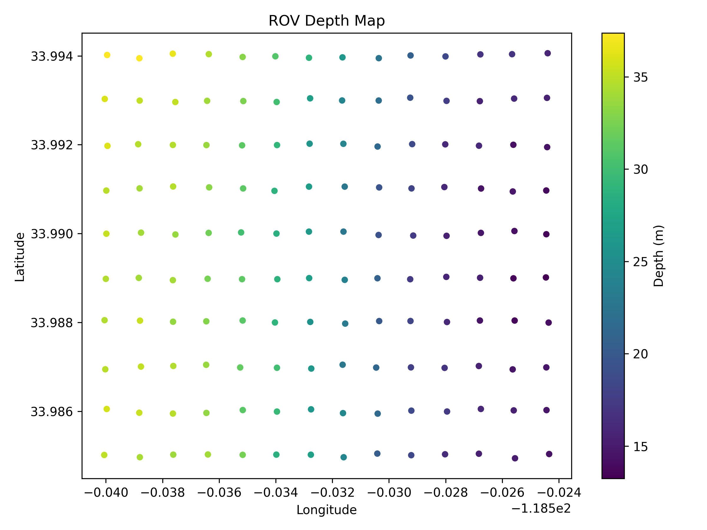
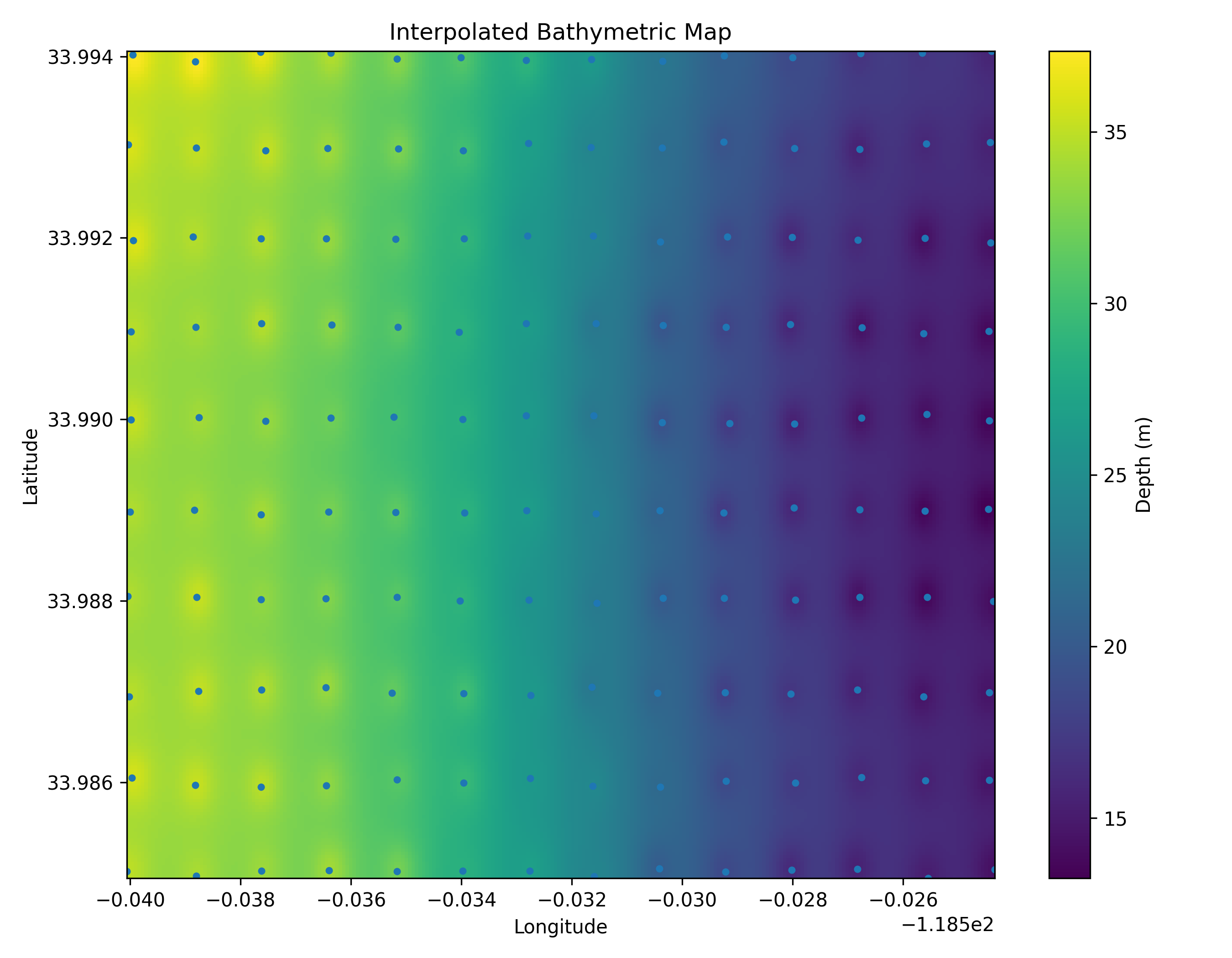
Interpolated Depth Soundings.

The bathymetry-sounding.json envelope is generated thousands of times per hour by the sensor's active sonar pinging the lakebed. Note the specific metric bathymetry-depth: 12.4m encoded in the strict SenML format.

Execution: The gateway consumes these disparate envelopes and stores them as massive arrays of raw coordinate points in SQLite. The Mission Portal then queries these points and executes an Inverse Distance Weighting (IDW) interpolation algorithm directly in the client's browser. This mathematics transforms discrete, scattered sonar pings into a beautiful, continuous 3D contour map, giving operators instant, real-time feedback on the topography of the unmapped ocean floor.

Offline Processing

Data Pipeline Scripts.

While the Mission Portal handles real-time IDW rendering, OMEGA also provides a suite of offline Python scripts for generating publishable scientific assets directly from raw CSV exports.

csv_to_png_depth_contours.py: Generates high-resolution, static 2D heatmaps with distinct topological contour lines using matplotlib. These static PNGs are designed for inclusion in formal academic papers.
csv_to_kmz_depth_overlay.py: Takes the interpolated depth arrays and projects them over satellite imagery, packaging the result into a compressed KMZ file. This allows marine biologists to drag-and-drop the 3D bathymetric overlay directly into Google Earth Pro for geospatial fusion with historical coral reef datasets.

scripts/csv_to_png_depth_contours.py

import numpy as np
import matplotlib.pyplot as plt

def build_grid(points, grid_size, power):
    lats = np.array([p["lat"] for p in points], dtype=float)
    lons = np.array([p["lon"] for p in points], dtype=float)
    depths = np.array([p["depth_m"] for p in points], dtype=float)

    lon_min, lon_max = lons.min(), lons.max()
    lat_min, lat_max = lats.min(), lats.max()

    # Generate the empty raster meshgrid
    xi_vals = np.linspace(lon_min, lon_max, grid_size)
    yi_vals = np.linspace(lat_min, lat_max, grid_size)
    xi, yi = np.meshgrid(xi_vals, yi_vals)
    
    # Execute IDW Math
    zi = idw_interpolation(lons, lats, depths, xi, yi, power=power)
    return lons, lats, depths, xi, yi, zi, lon_min, lon_max, lat_min, lat_max

def render_contours(xi, yi, zi, lons, lats, levels=12, output_path="map.png"):
    plt.figure(figsize=(9, 7))
    
    # Render the base color heatmap
    filled = plt.contourf(xi, yi, zi, levels=levels)
    
    # Overlay crisp contour lines on top of the heatmap
    plt.contour(xi, yi, zi, levels=levels)
    
    plt.colorbar(filled, label="Depth (m)")
    
    # Scatter plot the actual raw sonar ping locations 
    # to show where the interpolation occurred
    plt.scatter(lons, lats, s=6.0)
    
    plt.xlabel("Longitude")
    plt.ylabel("Latitude")
    plt.title("Bathymetric Contour Map")
    plt.tight_layout()
    plt.savefig(output_path, dpi=300)
    plt.close()

bathymetry-sounding.example.json

{
  "spec": "omega-wave.observation-envelope/1",
  "message_id": "bathymetry-example-0001",
  "message_type": "observation",
  "origin": {
    "node_id": "urn:omega-wave:node:survey-a:vessel-01",
    "device_id": "multibeam-sonar-main",
    "capability_ref": "https://example.invalid/omega-wave/things/survey-a-vessel-01-multibeam.td.json",
    "firmware_version": "0.2.0"
  },
  "routing": {
    "priority": "normal",
    "ttl_s": 86400,
    "ack_mode": "gateway",
    "max_hops": 8
  },
  "sample": {
    "sampled_at": "2026-04-18T19:00:00Z",
    "sequence": 1,
    "location": {
      "lat": 36.801,
      "lon": -121.79
    }
  },
  "tags": {
    "site": "survey-a",
    "platform": "survey-vessel",
    "medium": "water",
    "station_name": "Survey Vessel 01"
  },
  "payload": {
    "mode": "senml",
    "content_type": "application/senml+json",
    "schema_ref": "urn:ietf:rfc:8428",
    "records": [
      {
        "bn": "urn:omega-wave:thing:survey-a:vessel-01:multibeam/",
        "bt": 1776548400
      },
      {
        "n": "bathymetry-depth",
        "u": "m",
        "v": 12.4
      }
    ]
  }
}

Data Standards

CF-Compliant NetCDF Pipelines.

Scientific data is fundamentally useless if it is trapped in proprietary formats. OMEGA is designed for institutional interoperability and strictly adheres to the Climate and Forecast (CF) Metadata Conventions (cf_metadata.py).

Execution: All raw JSON/TLV telemetry collected by the edge nodes is eventually serialized into massive, multi-dimensional NetCDF arrays (cf_netcdf.py). These arrays include rigorous metadata describing the exact sensor used, the calibration date, and the QA/QC flags. This allows the data to be seamlessly ingested into national supercomputing repositories (like NCEI) for long-term climate modeling archival.

4D Data Arrays

Copernicus 4D Data Cubes.

The gateway does not just read flat CSV files; it is engineered to parse true 4D data cubes (Latitude, Longitude, Depth, Time) using the copernicus_cube.py architecture. These cubes represent terabytes of oceanic modeling data.

Relevance: By accessing the Copernicus Marine Service APIs, the OMEGA gateway extracts specific slices of this data cube. This allows the visualization portal to render complex, volumetric slices of ocean salinity and ocean color (Chlorophyll-a), and mathematically overlay the exact 3D physical position of the edge node directly inside the simulated data cube.

Model Validation Skill Score

The portal's Copernicus sea-surface-temperature model is statistically validated against the independent NOAA observation network, achieving strong agreement with a correlation of r = 0.971 and an RMSE of 0.774 °C across 12 independent stations.

Scatter plot of OMEGA model sea-surface temperature versus NOAA observations, correlation r = 0.971

Mission Portal & AI.

Engineering Reality: The Fiji → Hawaii Dateline Bug

The Glass Bridge Interface.

4D Temporal & Z-Axis Engine.

Master Time Clock

Z-Axis Slicer

Absolute Data Purity.

Operational Workspaces.

Live Observatory

Predictive Simulation

Data Library

Engineering Deck

Public Federation

Digital Twins & UI State.

QARTOD Quality Control Math.

Bathymetry & IDW Math.

Fast Fourier Transforms (FFT).

Signal Preparation

Time to Frequency

Harmonic Dampening

The ~100-Tool Action Registry.

Global Federations

Fishing & SAR

UI Automation

Natural Language to Geo-Bounds.

Absolute Read-Only Execution.

The Query Preprocessor.

Auto-Execution Overrides.

IDW & Kriging Algorithms.

Inverse Distance Weighting (IDW)

ETOPO Fallback Grid

Executing IDW in Python.

Acoustic Sounding Cones.

Interpolated Depth Soundings.

Data Pipeline Scripts.

CF-Compliant NetCDF Pipelines.

Copernicus 4D Data Cubes.

Model Validation Skill Score